While many people use my Blender shaded relief tutorial, and associate me with the software, I’m really not much of a 3D cartographer. I make oblique-view maps only rarely, and when I do, it’s usually in a simplified, abstract style, rather than the detailed, naturalistic representations that people like Tom Patterson produce. Here’s a not-quite-finalized draft that I’ve been working on for a client’s book.

I make oblique views in this style mostly because they’re much easier and faster to produce than a more realistic terrain view (one with trees and shimmering water and clouds) — they fit well in projects where a client needs a 3D view, but there isn’t the time or budget to produce something very detailed. Also, I make these because I’m not yet particularly skilled in making the fancier realistic maps, though I’ve made some attempts.
So, let’s walk through how I make one of these. There’s a lot to cover, but once you get the hang of it, they’re not too complicated. And, if you want to work your way toward eventually making more photorealistic terrain renders, much of what we discuss here will be useful to you.
This tutorial presumes that you’re familiar with the basics of using Blender and that you’ve gone through my shaded relief tutorial or something similar. It also presumes some familiarity with the basics of Photoshop or other raster image editing software.
To keep things simple, we’re just going to pick right up where we left off in my previous tutorial. You could start from scratch, but I find it easier to just load up an old shaded relief Blender file, change out the DEM, and make use of some of the work I’ve already done. So, go ahead and set up everything like you were preparing a shaded relief: load in the DEM you’d like, get your plane resized, etc.
Camera Setup
If we want to make an oblique view, the first thing we’ll need to do is set up the camera; the settings that we were left with from the shaded relief tutorial aren’t quite right for this job. The camera is in the wrong position (looking straight down at our terrain), and it’s got the wrong lens. If you remember from Part 4 of the previous tutorial, we had to switch our camera from a perspective to an orthographic view, to avoid perspective distortions that would make our shaded relief look weird. Now it’s time to switch it back. We need the more realistic perspective view here; we want our camera to operate more like an ordinary real-life camera that most of us would use.
So, select your camera, then head on over to the Object Data Properties panel by clicking the green icon of an old movie camera on the left of the panel. Then change the lens type to Perspective.

Next up, we need to reposition our camera. Right now, you’ll see it’s pointing straight down at the terrain, because that’s what we needed for our shaded relief. But, for an oblique view, we want to be looking at the terrain from an angle.
Getting the right view takes some trial and error, and some exploration. You’re going to reposition the camera and change its orientation, eventually finding the place you’d like. If you select your camera the choose the Object Properties panel (the orange square), you can adjust the Location and Rotation of your camera by plugging in whatever numbers you like, or by clicking on a number and dragging your mouse left/right. Play around with those for a moment to get comfortable. As you change the numbers, look at the 3D Viewport to see how the camera moves around.

But how do you know if it’s in the position you want? We can’t see the terrain, just a flat plane. You could make test renders over and over again, but that takes a lot of time. Instead, let’s look at a rough version of the terrain. At the bottom of the 3D Viewport (or maybe the top; it seems to move around when I look at Blender on other people’s computers), you should see some icons of spheres. If you mouse over them, they’ll probably say something about “Viewport Shading.” Click the last one of the four icons, that looks like a sphere with little shadow lines.

Don’t see the icons? No problem. Click on that bottom toolbar with your middle mouse button (or alt + left button, if you’ve turned on 3-button emulation in the last tutorial), and drag it until you find the icons.
Now in your 3D viewport, you should see a rough rendered version of your terrain. It may look comically exaggerated — the level of vertical exaggeration needed for shaded relief is usually much higher than will look realistic in an oblique view. So, you may want to tone that down until it looks right (remember that’s by adjusting the Scale property of the Displacement node on your plane’s material).

Now that we can see our terrain, figuring out where to put the camera gets a little easier. You may remember from the last tutorial that we have a shortcut for looking through the camera’s lens to see what it sees. To do this, find the View menu, choose Cameras, then Active Camera. You can also hit 0 on the numeric keypad.
Now you see what the camera sees, and as you change its position, you can start to home in on the area you want to look at. Take a minute to play around and get closer to the terrain (but don’t go to the trouble of finalizing your position yet; we’ll talk about some tools that will help make that easier).

In the 3D viewport, you’re only going to see a simplified terrain, since Blender is trying to quickly show this to you on the fly, rather than doing a fully detailed render. Blender is also simplifying your DEM, cutting out a lot of details to make it render faster. But, as we zoom in, it doesn’t get more detailed. It would be nice to see a less-simplified terrain so that we can fine-tune our camera position. An easy way to do that is to go back to those Viewport Shading buttons (the four spheres) and click on another sphere to switch to another mode (any of them will do), and then switch back to Rendered mode (the 4th sphere). Notice how more detail comes in.

Why does turning the Rendered view mode off and on again help? Well, when we first turned Rendered mode on, your camera was probably far from the terrain. And Blender said, “I’ll load in just enough of your DEM data to make this quick preview look fine at that distance.” And as we zoom in, it didn’t update the level of detail to fit out new camera position. So, by turning the mode on and off, we force it to re-evaluate how much of the DEM detail that it needs to load in. Note that, no matter where your camera is, Blender will always use the full detail when you’re doing a final render by going to Render→Render Image as we normally do. What I’m talking about here is just about Blender’s attempt to show you a quick preview in the 3D Viewport with as little data as possible.
Now, there’s one other way to move the camera around which you will probably find useful. Instead of plugging in numbers, you can click and drag around the scene. If you press G (for “grab”), and move the mouse, you’ll start moving the camera around the scene (make sure you’ve got the camera selected and not the plane; I often make that mistake). This can help you position things. Hit Enter to finish grabbing, or hit escape to go back to your old position. If you stop moving a moment, Blender will catch up with you and fill in a more detailed rendering.

Another useful tip: you can constrain movements when you grab things. Let’s say you want to move the camera to the left. It’s hard to do that when grabbing, because your mouse might slip and you might shift up or down. It’s also not really possible by adjusting the Location values for your camera, because shifting your view left/right would require adjusting both the x and y position of the camera (since your camera is pointing at the terrain at an angle). The solution for this is to use shortcut keys that constrain our camera movement. Hit G to grab, and then hit X. Notice near the bottom of the screen you’ll see a message that says “along global X” — this means that now, you can only move the camera along the X direction of our entire scene. You may even see a line show up on screen showing you the X-axis of the scene, and if you try to grab, you’ll only move along that line.

Hit X a second time. Now the message says “along local X.” Now our grab movement is constrained to the X-axis of our camera’s view, not the entire scene. A line will probably show up, showing you where you’re constrained to. As you drag the mouse, note that you can only move left/right.
Constraints like this are really handy to position your view right where you want it. There are also constraints for the Y and Z directions. Moving along the global Z would be raising/lowering your camera relative to the terrain. Moving along the local Z would be pushing your camera forward or pulling it back along the direction it’s facing, effectively zooming into the terrain or zooming out.
There are still more constraints you can use, if those aren’t enough. While grabbing, if you hit Shift-X (or Shift-Y/Shift-Z), you can lock a direction. So, for example, you could allow your grab action to move the camera, but lock your global Z, so that it never gets any higher or lower in its elevation above the terrain. And you can hit Shift-X (or -Y or -Z) twice to lock the local direction, rather than the global one.
Finally, besides grab, you may want to also try pressing R to rotate the camera. This operates just like grab, letting you drag the mouse around to change the camera’s orientation, and you can likewise constrain yourself to (or lock) any axis you want. I don’t use this one as often, but it can be handy. Usually I rotate the camera by plugging in specific numbers, though, as it’s easier to wrap my brain around.
Ok, that’s a lot to take in, so I encourage you spend a little bit of time messing around with all those options and getting comfortable moving around.
Now, what if you’re unhappy with the shape of your camera’s window on the terrain? Well, that’s tied directly to your final render size. When we were doing shaded relief, we set it the same size as our plane. But here, it can be anything you want! Head on over to the Output Properties panel and adjust the X & Y resolution of your image. Remember, that’s the icon that looks like a photo coming out of a printer. Your camera view will change as you adjust your output dimensions.

Ok, now that you’ve got that set, it’s finally time to set up our actual terrain view. Using the grab/rotate tools, and/or plugging in numbers on the camera’s Object Properties panel, get your camera positioned where you’d like it. You might also decide at this point to tweak your terrain’s vertical exaggeration, as it might look too high or low as you get close to it. It’s an iterative process to get things looking right.
Here’s where I ended up with my own terrain: a 16:9 aspect ratio, with some mountains on the left side and valleys on the right.

If you’d like, you can do a render of this right now to see it at full detail (or as much detail as your DEM supports — since you’ve zoomed in so much on the terrain, your DEM will need greater resolution than if you were viewing the whole thing from far above). Mine’s looking pretty smooth — about as smooth as the quick preview in the 3D viewport, really. But, for my tutorial purposes, that’s going to be just fine. And, for a lot of cartographic purposes, simplified terrain is preferable to detailed terrain.

Now, what we’ve just done here — getting the camera set up — is the starting point for basically any oblique-view map you want to make, whether it’s the simplified look that I showed you at the start of the tutorial, or it’s a photorealistic render with beautifully detailed trees, clouds, and streams. But we’re going to stick to the simplified look.
Depth Map
The main reason I use Blender to render shaded relief is that it lights the terrain realistically. To do this, it calculates the path of light rays coming into the terrain and bouncing around, the way real light does. That’s something 3D software can do that a more traditional hillshade algorithm can’t. Likewise, you can use Blender (and similar programs) to create highly-detailed, lifelike oblique terrain maps, because it has this capability of simulating realistic lighting and materials, down to the level of giving each individual tree its own shadow.
Now we’re going to take all those powerful capabilities and completely ignore them. We won’t end up caring at all what our final render looks like. If you felt like it, you could even go delete your light source right now from this file, because we won’t need it (though it would be hard to position your camera correctly in the dark).
The main thing that we need from Blender, instead, is a depth map. Put simply, this is an image that encodes how far from the camera our terrain (or other object) is. Here’s the example from that linked Wikipedia article, by user Dominicos:

On the left is an ordinary 3D view of a cube, with lighting and shadows and such. On the right is a depth map. Darker areas mean that the cube is closer to the camera. Lighter is farther away. Here’s an example with my chosen terrain view:

In the depth map on the right, you can see how the closest mountains are darker, and the scene fades away into white as it gets farther back. This, by itself, is pretty visually interesting and fun to play around with. But it’s just our starting point.
Now, since the depth map just shows us what’s near and what’s far away, our lighting and materials don’t really matter. If you removed the light from this scene, or changed the color of the terrain, that wouldn’t change how far away the mountains are from the camera.
So, let’s get Blender to give us a depth map. First off, we’re going to tell it to start calculating the depth every time we render things. It doesn’t necessarily do this by default. Head on over to the Layer Properties panel (the icon that looks like a stack of images), and go to Passes→Data, then check Z. A “Z Pass” is another name for a depth map.

Next, you’re going to want to go to the Compositor window. To get there, click down in the bottom corner, in the same place you’ve previously used to change between the Shader Editor and the 3D Viewport. Once you’re there, check the box for Use Nodes.

Once you get there, you should see something that looks somewhat familiar. The Compositor looks a bit like the Shader Editor, in that we can plug various nodes into each other, which instructs Blender to carry out certain operations. The difference here is that the Shader Editor was all about setting up the material our plane was made from, and adding terrain to it. The Compositor is a window used for post-processing. It acts much like Photoshop and other raster image editing programs. Once Blender is done making a rendered image, you can use this window to have it do all sorts of things, like adjusting colors, mixing images together, adding filters, and so on.

The big box on the left represents our rendered image, and right now the image output is connected to the image input of the Composite node. This just means “take the image of the render, and then send it directly into the final image output location, without any changes.” It just makes sure your rendered image, with all its fancy lighting, shows up at the end.
You may notice the Depth output on the Render Layers node. This is our depth map, exactly what we’re looking for. When Blender renders a scene, it also calculates the depth map for that scene. But how can we see it? Well, let’s plug that Depth output right into the Image input, so that instead of seeing our terrain render at the end, we see our depth map. Now render your scene; you should see the render at first (while Blender calculates all that realistic lighting that we no longer care about), but at the end it will get replaced with the Depth map, because we’ve told Blender that’s what we want as our final image.

Before we go any further, let’s take a moment to make this whole process go faster. You might remember that render time is related to the number of render samples — more samples look better, but take more time. It can take several minutes to render a final shaded relief image. A photorealistic terrain map might take hours to render. But, we don’t care about a good-looking output, and it turns out that Blender only needs 1 render sample to generate the depth map. So, head on over to your Render Properties tab, and turn down your render samples to 1. From now on, all our test renders will go much faster.

Now, you may notice that my initial depth map doesn’t darken all the way to black. The nearest mountains are kinda grey. We’ll need to fix that, because it represents lost information. If we used the entire black-to-white range, we’d be able to encode a lot of different depths, because there are a lot of different shades of grey in between black and white. If we instead had a depth map that was only grey to white, there are fewer shades of grey in between, and so we can’t encode as many differences in depth.
To fix this, we need to add a new node. Hit Shift-A, and use the search bar to look for Normalize. Stick that new node in between our two existing nodes, like so:

This tells Blender to take all the depth information that it’s calculated, and then map it onto a black-to-white scale (I believe that, behind the scenes, it’s really a 0 to 1 scale that eventually gets mapped onto a black-to-white raster once it knows the bit depth of your output, but that’s more detail than we need to go in to). If we render again, we get the full greyscale range.

Finding Edges
Now let’s turn this into something that looks more like terrain. To do that, we’re going to find edges in our image. If you’ve played around in Photoshop, you may have seen a tool that does that: it looks for places where the colors in your image shift suddenly. Blender has tools like this, too. In our depth map, a sudden shift in color means a sudden shift from something close to something far. On the lower left of the image above, you can see we have a dark foreground mountain, and then right behind it a mid-grey mountain some distance behind it, so that’s a sharp transition from foreground to background. If you imagine drawing lines that trace along those transitions, you’d start to outline the shape of each mountain or ridge as it occludes the terrain farther behind it.

To get Blender to do this for us, we’re going to set up a Filter node. Just like with Normalize, just hit Shift-A and then search for Filter. When you place the node it will have a different name, like “Soften”; that’s fine. Plug it in after Normalize.

Notice that on the Soften node, there’s a dropdown menu that also says Soften. Click that and choose Sobel. Notice that the name of the node now changes to Sobel. So, this is really a Filter node, but it happens to name itself after whichever particular filter you’ve chosen. Just like Photoshop or GIMP or other raster image editing programs, Blender has several filters to choose from that can modify how your image looks. The Sobel filter is one that detects edges, and it’s named after one of the people who invented it. Now that you’ve got it plugged in, do another render.

Those light areas are our image edges. The brighter they are, the bigger the shift in color in our image (which means, in our case, the bigger the shift in depth). You can see how it effectively outlines the tops of ridges, and even filled in some details on the sides of mountains.
While it has a cool, glowing, light-on-dark effect, let’s reverse that and have the edges be black and the background white. Add an Invert node after the filter:

Now it’s switched. Some details are perhaps a little harder to see, in the areas with weaker edges, but we can work on that later.

The Sobel filter is only one way of detecting edges. Another one on that list, the Kirsch filter, also does so. Switch to that one and have a look at your rendered output.

It’s pretty similar, though to my eye it seems maybe a little darker and more emphatic about each edge. But I think there’s also a little less distinction among the hardest edges. I’m no expert on these, and I’m sure a specialist could do better in pointing out the aesthetic differences and their relative merits.
Save your filtered depth map. You can pick your favorite, Sobel or Kirsch, or even choose both. When you save, make sure to choose a Color Depth of 16. This will store our images with 16-bits of data per pixel. This is important, in that it lets us encode way more information (basically, way more levels of grey). That’s important because we have a lot of faint areas we’ll want to work with. By storing a lot of levels of grey, this means that even those faint areas are actually still made up of many separate (if barely distinct) shades. So later on we can darken them and accentuate their differences without losing detail.

Photoshop Manipulation
Now we start doing some manipulation on these images in Photoshop. Other programs will do this stuff, too, so feel free to translate these concepts into GIMP or whatever other software you’re comfortable with.
It’s important to note that the steps I’m going to follow are sort of like a recipe — everyone who uses Photoshop for cartography does things a little differently, because they have their own taste and their own habits. I highly encourage you to play around and try doing things differently than I do, once you get the hang of it. Experiment to find your own style. I’m just showing you mine (which actually changed during the writing of this tutorial).
I’m going to be a little less detailed here as far as telling you what to click, because this is going to presume some Photoshop familiarity. This is partly because this tutorial is already getting really long, and also because, if you’re new to Photoshop, this is probably not the best tutorial to start with. I’d encourage you to first get comfortable with the software by watching courses on YouTube or the like. I was more detailed with the Blender portion because I know that’s much less familiar to most of readers and that’s where I think it’s much easier to get lost.
I picked the Kirsch filter for my image. At this point in the tutorial, I’m going to switch to a totally different terrain, too, because as I was writing, I realized that I should have chosen something a bit more detailed to better show off the method, so I called up an old file where I’d done this before (the one used in my initial example at the top of the post). Here’s my new, more interesting terrain. Still just made entirely of edges, though.

Next I’m going to soften the Kirsch image a bit with a simple gaussian blur (Filter→Blur→Gaussian Blur). I’m going to do a radius of 2 pixels, but your preference may vary. This gives the Kirsch a softer look that I prefer.

Next up, I’m going to add a Levels adjustment layer (Layer→New Adjustment Layer→Levels) just above the Kirsch, and use that to darken things a bit by dragging the left slider over. This will discard the lighter pixels and redistribute the remaining pixels along a black-white gradient, thus darkening things and bringing out some detail in the lighter areas (this is where having a 16-bit image helps a lot).

We’re already almost there. I’d like to take some of those faint foothills in the bottom of the image and darken them a bit more, though. So, I’m going to add another Levels layer, and I’m going to darken things again, until the just the foothills are how I want them.

Now, of course, everything else in the main mountain range is too dark. So, let’s constrain our second levels adjustment so that it only affects some areas. I’m going to go into its opacity mask, and paint in some black to mask it out of the higher mountains, so that it only darkens parts of my image.

Notice that I feathered mask quite a bit, for a smooth transition. Now my levels adjustment fades out as it gets into the mountains, and fades back in among the foothills. Remember, here’s what it looked like before:

You can keep going around making adjustments like that and tweaking as you like. In a previous version of this method, I used to stack Kirsch and/or Sobel filters on top of each other with various blend modes. You could also try using Curves instead of Levels for finer control. I leave this all as an exercise to you. Experiment!
Now, that’s our really basic, abstract terrain. But, there are a few other niceties we can apply if we like.
Depth Effects
To add the first of these niceties, we’ll need to go back to Blender and grab another layer. In your Compositor, disconnect the invert and filter nodes, so that you’re just outputting the original depth map. Then, save that.

Now, bring it into Photoshop and drop it into your file. This depth map can do a couple of things for us. If you think about looking at a real-life mountain scene, as things get farther from you they might get obscured by mist if the weather conditions are right. We can use the depth map to simulate that. This is something people do in photorealistic terrain renders all the time.

To add mist (or fog), we just need a new layer that’s solid white, and then we can use our depth map as the mask for that layer, making that white layer transparent near the front of our scene, but more opaque near the far end.

So now, as our scene recedes away, it gets fainter and mistier. You could adjust the opacity of the layer to tone down this effect. Note that I have the Depth layer turned off right now — it’s not visible, we’re just using it in the white layer as a mask.
I can also use this mask to simulate depth of field — making things in the background fuzzier, and focusing our attention on the foreground. In Photoshop, I select my Kirsch layer and go to Filter→Convert for Smart Filters. This lets me apply filters to it, but also mask them. Next, apply a gaussian blur to the layer, this time much stronger — say, 10 pixels or so.

Notice a new layer popped up, the Smart Filters layer. There’s one smart filter applied: the Gaussian Blur, which you can turn on and off. Copy your depth map into the Smart Filters mask.

Now the blur applies more strongly to the faraway places, and is less apparent nearby. You could once again tweak the strength of the blur, or adjust the darkness of the mask to further control this. This is another trick that you’ll find useful if you move beyond this tutorial toward more photorealistic renders.
In my case, I’m actually going to turn both the fog and blurring off, as that’s not the look I’m going for, but I wanted to show them to you.
Adding Other Data Layers
Now we’re all done with depth maps and their edges. You can get quite a lot out of a terrain image without even having to render lighting, it turns out. But, what if you want to stack some other data on top of this? Rivers, points of interest, and so on? To do that we’ll go back to Blender.
In your Compositor, reconnect the Image connectors of the Render Layers and the Composite nodes. In other words, put things back to the way they were — we want to look at renders again, rather than depth maps.

Now head into your Shader Editor. To add more data, you’re going to need another image that lines up correctly with your DEM. So, here’s my DEM, and here are some rivers that I’ve exported as a raster image (I was in Illustrator and saved them as a .png).

The spatial boundaries of each image are the same — they layer perfectly atop each other in space (they can be different resolutions, though). You may need to do a little preparatory work to make sure everything is aligned.
Now, let’s go into our Shader Editor for our plane. This is where, in the past, we’ve done things like set our vertical exaggeration and such.

You may recall that we talked a fair bit about the Principled BSDF in the last tutorial. This is the node that tells Blender how light will interact with the surface of our terrain — how it bounces, how it absorbs, etc. You may have played around with adjusting the Base Color parameter, or even plugged an image into that connection point, as mentioned near the end of the tutorial. Let’s give that a try: hit Shift-A to add a new node, and search for the Image Texture node. This is something you’ve done once before: you added the DEM as a displacement texture long ago when you set up your original shaded relief that we based this all on. Load your rivers (or points of interest, or whatever other layer you want to add in) into the image texture and plug it in to the Base Color.

If I set things up like above, I’ll get this as an output, showing where my rivers are in the oblique view.

This is somewhat useful, but there’s a problem: while it has the rivers that we want, it’s also got a shaded representation of the terrain, too. I want to add just the rivers to my existing simplified terrain that I’ve created from those edge filters. However, there’s no easy, clean way to pull the rivers out of the image above and ignore the rest (you might try selecting by color, but it’ll be a pain in many cases). Most of the time, the best we could do is bring it into Photoshop, then use it as a reference to manually trace the rivers in a new layer, then throw it out. Now, that’s a perfectly serviceable way of doing things (and not uncommon), but let me show you a better way that’s faster and more useful.
Go back to your Shader Editor, and get rid of the Principled BSDF, and replace it with an Emission shader. (Shift-A, then you can search for it). Plug it in exactly the same was as the Principled BSDF was connected.
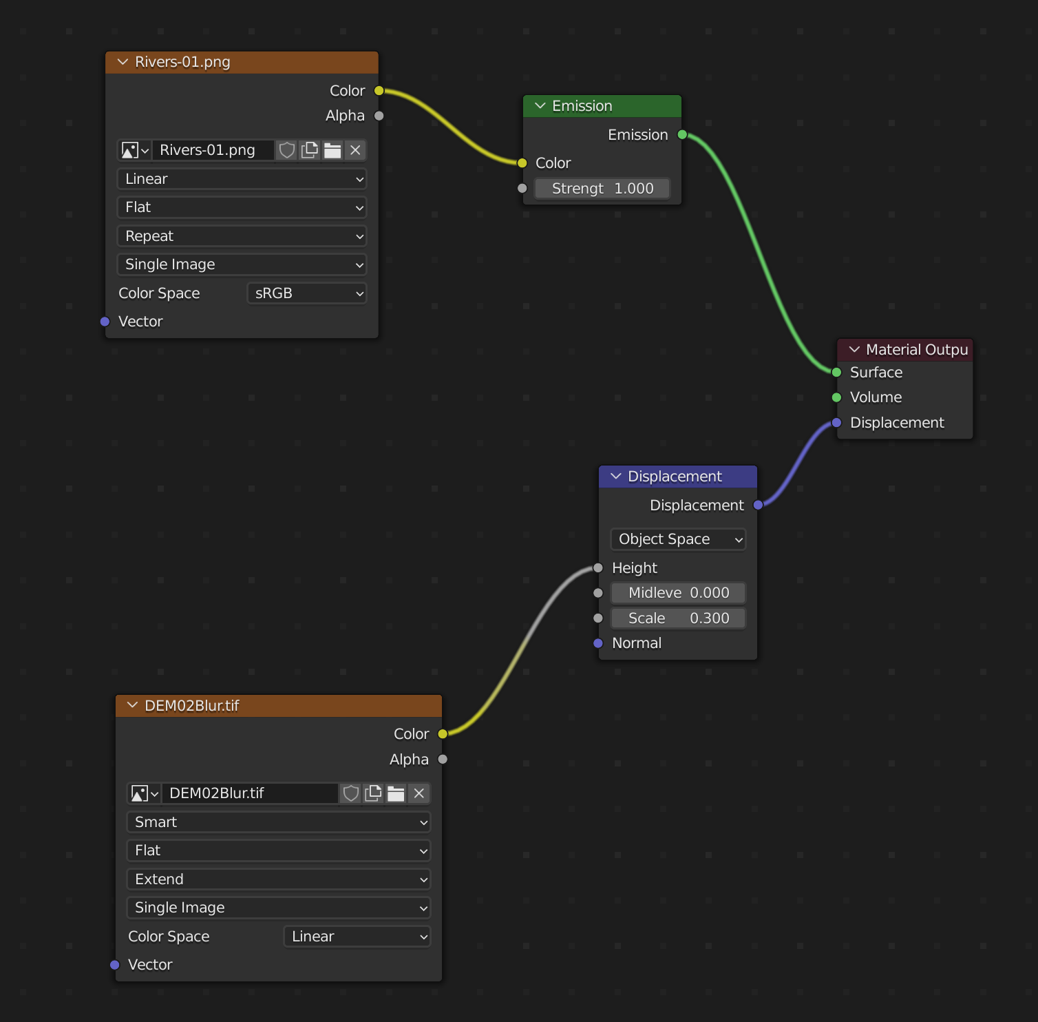
So, what does all this mean? Well, an Emission node changes your terrain plane. Instead of having a solid material surface that light can bounce off of, it instead is now going to emit light in your scene, a light that is unaffected by shadows or other such complexities. And the light it emits is going to look like my rivers layer, since that’s the image that’s plugged into the color node. And, best of all: you can keep your render samples at 1. Emission nodes only require one pass. So, this will speed us up again, vs. the slower method of using the Principled BSDF to make a reference layer. Here’s what I get when I render:

Just the rivers, with nothing else. All the colors are the exact same as my input file, too, and I don’t have to worry about the lighting settings changing them, as I would if we’d used the Principled BSDF. Now I can take this over to Photoshop, drop it on top, and either select/delete the white pixels, or just set the blending mode Multiply (white pixels disappear in Multiply).

Again, everything lines up perfectly, because the original layers I used in Blender (my DEM and my rivers image) both covered the exact same spatial extent.
The downside is that it’s not easily editable — any adjustments that you make to your data layer have to be done to the image you’re feeding into Blender, and then you need to re-render. Fine-tuning can be a pain, and things can look pixellated (since this is all based on raster images). As such, even using this Emission method, it’s still common to just treat this as a reference layer and trace out the data, just like with the earlier method using the Principled BSDF. Nonetheless, the Emission method is quicker to render and at least lets you add your data cleanly to the map to make tracing easier, if you have to trace.
Here, for example, is that same image with a manual vector tracing in Illustrator. So now I have vector rivers atop the terrain we made earlier, which are easier to fine-tune if the style needs to change.

Instead of adding in vector data, what if we did raster data? The Emission method enables us to easily add a color layer, line hypsometric tints, land cover, or imagery to our map. Instead of plugging my rivers in as my color layer, let’s instead plug in my DEM as the color layer.

Remember, your DEM is represented in Blender as a simple black and white image, with black being low and white being high. Here’s what that renders:

Again, it’s just emitting the color of the DEM, and nothing more. But this is a pretty useful layer. Let’s bring that into Photoshop and drop it atop everything else. Now I can blend it into the rest of the layers. Here, I’ve set it to Multiply, with a 70% opacity.

Obviously, there are lots of options for blending here, and a lot of different directions you could take it. I could, for example, colorize my hypsometric tint first using the Gradient Map adjustment layer:

Gradient Map converts a black and white image into whatever color ramp you’d like. Note that I made sure to apply the gradient map only to the hypsometric layer, by Alt-clicking the space between the adjustment layer and the hypso layer to get that little arrow to turn on. Now when I blend that in with Multiply, I get this:

Instead of feeding your DEM into the Emission node in Blender, you could do a land cover layer, instead, or satellite imagery. Whatever you want to load into the color slot of that node, yields you something you can drop in with Photoshop, whether it’s raster data or (rasterized) vector data.
There are a lot of directions you can take this, and I could keep going on, but this is already running pretty long and there’s a lot to digest here, so I’ll wrap up for now. Thanks for playing! And thanks to all my patrons who keep content like this going! If you’d like to support my efforts, you can donate via the links below. Also, just spreading the word about my work is a big help!
Bonus Addendum
I mentioned earlier that the Compositor gave you a lot of options such as you might find in Photoshop. Just to demonstrate that further, I spent a while poking around Blender (after releasing this tutorial) and found a node setup that would give you a similar result without using Photoshop.

I won’t go into detail here, but it largely puts the image through the same stack of processes as our Photoshop layers. I will leave this as an exercise for you to explore on your own, if you like. I would say that the process felt more clunky to me than doing it in Photoshop, though that’s likely just because I’m not as comfortable in Blender.
